Introduction:

I accelerate an existing Python codebase while avoiding a full rewrite to keep the interface, visualization system, and data formats in tact. First I use cProfile to determine the function that consumes the most compute time. Next I implement a parallelized mathematical equivalent of the bottleneck function using concurrency facilities in modern C++ and achieve intra-process concurrency. I write a script to compile and test this function into a Python-importable module using PyBind. I then modify the original Python codebase to import and call the C++ function when requested from the command line. Lastly I measure an up to 3X performance improvement and provide observations.

Initial Execution:

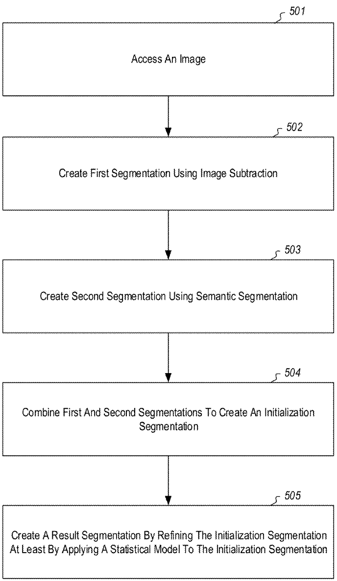
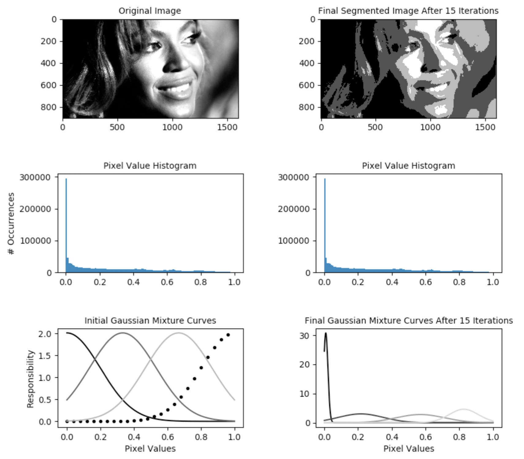
The Python codebase we want to accelerate is an estimator for Gaussian Mixture Models (GMM). I’m interested most in the heart of the algorithm itself. The visualization system is useful for research purposes, but for production purposes it does not need to run. For that reason, I start by running the following command line which disables visualization and executes only the mathematical implementation of the estimator:

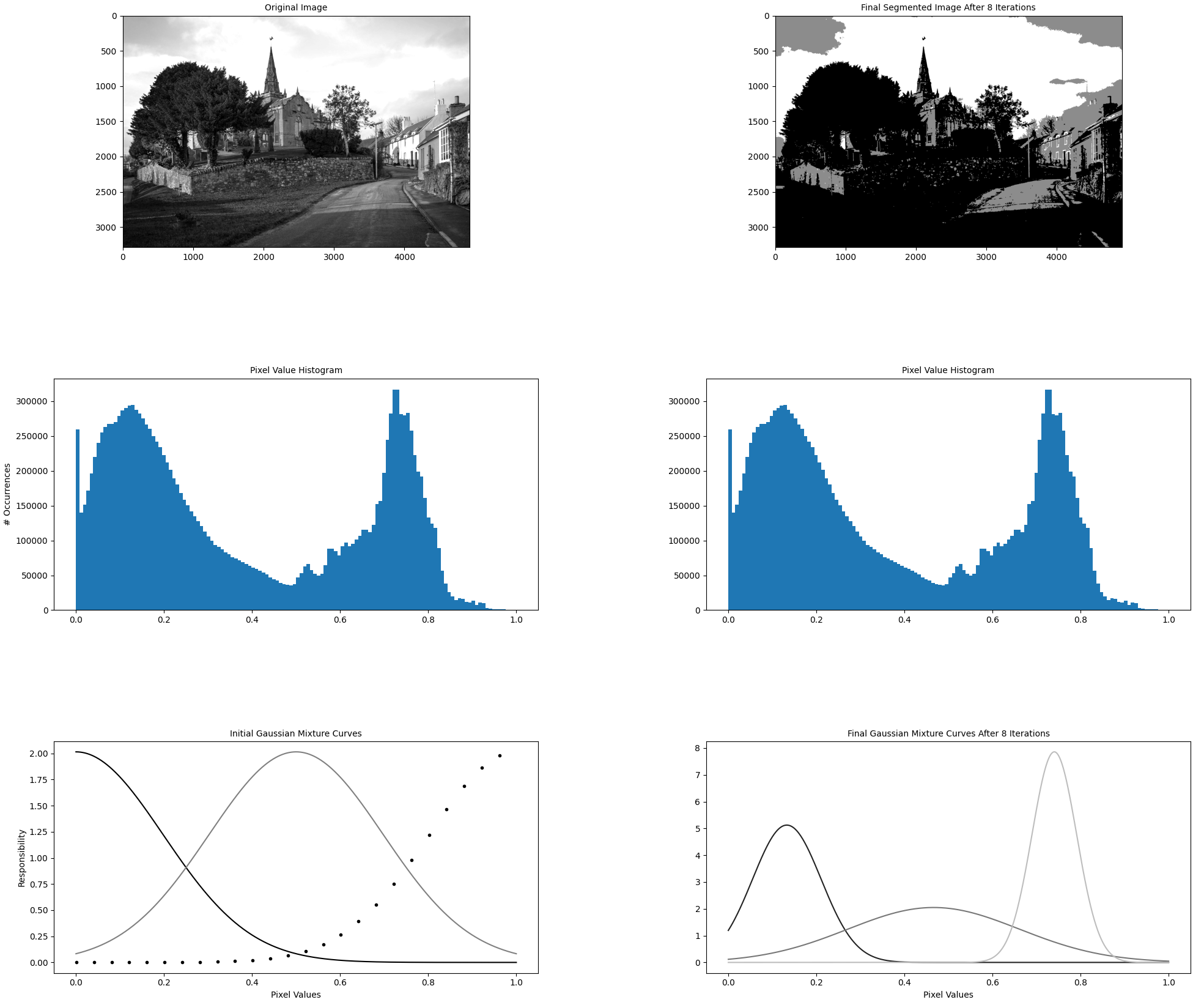
time python3 gmm_segmentation.py --first-image=example_data/church.jpg --components=3 --iterations=8 --visualization=0 --precompiled-num-threads=0

The driver function of the codebase is in the file gmm_segmentation.py which is where our efforts will go. --first-image specifies the location on disk that contains the image for which we want to compute a GMM. We will keep it constant. The algorithm hyperparameters --components and --iterations are hand-selected and not relevant for this article. While they do influence algorithm runtime (runtime increases as the number of components and iterations increases), we will keep them constant at all times. As discussed, --visualization toggles the visualization capability which outputs figures explaining the algorithm state as shown below. --precompiled-num-threads toggles the use of the accelerated C++ function. We will start with this parameter set to 0 meaning we run only the original Python implementation.

Observations upon Initial Profiling:

I insert cProfile calls inside the main() function of gmm_segmentation.py. The profiling capability is compact requiring only two lines to construct and enable the profiler before the business logic gets executed and 5 lines to summarize and display the results afterward. The function calls initialize_expectation_maximization() and execute_expectation_maximization() contain all of the logic we want to profile.

Upon executing the command line in the previous section on an AMD 3975WX CPU, we see the following (abridged) output:

   ncalls  tottime  percall  cumtime  percall filename:lineno(function)
       16   12.900    0.806   36.050    2.253 /home/a/gmm/gmm_segmentation.py:109(compute_expsum_stable)
      241    8.690    0.036    8.690    0.036 {method 'reduce' of 'numpy.ufunc' objects}
       48    5.702    0.119    5.702    0.119 /home/a/.local/lib/python3.10/site-packages/scipy/stats/_continuous_distns.py:289(_norm_pdf)
        8    4.791    0.599   22.844    2.856 /home/a/gmm/gmm_segmentation.py:176(compute_expectation_responsibilities)
       48    4.131    0.086   15.788    0.329 /home/a/.local/lib/python3.10/site-packages/scipy/stats/_distn_infrastructure.py:2060(pdf)
       48    3.042    0.063    3.042    0.063 {built-in method numpy.core._multiarray_umath._insert}
        1    2.623    2.623   44.719   44.719 /home/a/gmm/gmm_segmentation.py:209(execute_expectation_maximization)

real	0m45.572s
user	0m37.171s
sys	0m18.049s

The profiler recursively measures the time consumed by the functions that get called between the profiler.enable() and profiler.disable() calls. The functions are displayed in decreasing order of compute time consumed. Due to recursive operation, if functionA() internally calls functionB(), time spent in both functions is considered in the profiler ranking even though the profiler is only enabled and disabled once.

We see that the hottest function is compute_expsum_stable() in gmm_segmentation.py. Along with NumPy operators, we see also that compute_expsum_stable() calls a SciPy function, scipy/stats/_continuous_distns.py:289(_norm_pdf) (a.k.a scipy.stats.norm.pdf() in the actual code), which is listed as the third hottest. Therefore I decide to re-implement compute_expsum_stable() in C++ with hopes of increasing its performance.

Implementing, Compiling, and Importing a Custom C++ Module

NB: To illustrate this without the complexity of the GMM codebase, I made a separate and compact repo https://github.com/alexhagiopol/pybind_examples with no other purpose.

A multithreaded C++ equivalent of compute_expsum_stable() is implemented in computeExpsumStable() in PrecompiledFunctions.cpp. The re-implemented function is mathematically equivalent to the Python original and calls no external math functions other than basic matrix element access operators from the Eigen library. If using only a single thread, I expected the C++ function to underperform the Python version because the C++ function (a) naively re-implements SciPy’s scipy.stats.norm.pdf() without care for memory alignment or other lower level optimizations, (b) the original Python code uses vectorized syntax, and (c) the large 3D matrix P must be copied twice when calling the C++ function due to Eigen’s lack of official support for 3D matrices.

To compile the C++ code, the CMakeLists.txt file defines the build procedure for the Python module precompiled_functions which will land in a build folder precompiled_functions_build. The file re-uses PyBind’s own CMake module generation function. The Python script build_precompiled_functions.py automates the build process from build folder generation, to CMake invocation, to binaries generation. The Python module is imported by gmm_segmentation.py in the initialization of the GMM_Estimator object. The Python implementation of compute_expsum_stable() calls either a pure Python implementation or the imported C++ implementation depending on the user’s selection in the --precompiled-num-threads command line parameter. If set to 0, the pure Python implementation of compute_expsum_stable() will run. If set to 1 or more, that many threads will be given to the C++ implementation instead.

Observations upon Second Profiling:

With a C++ equivalent of the hottest function implemented, we give it one thread and do a second profiling run to compare against the pure Python version:

time python3 gmm_segmentation.py --first-image=example_data/church.jpg --components=3 --iterations=8 --visualization=0 --precompiled-num-threads=1

results in the following (abridged) profiler ranking:

   ncalls  tottime  percall  cumtime  percall filename:lineno(function)
       16   25.568    1.598   25.568    1.598 {built-in method precompiled_functions_build.precompiled_functions.computeExpsumStable}
        8    4.878    0.610   19.853    2.482 /home/a/gmm/gmm_segmentation.py:176(compute_expectation_responsibilities)
       16    4.394    0.275   29.962    1.873 /home/a/gmm/gmm_segmentation.py:109(compute_expsum_stable)
        1    2.769    2.769   38.986   38.986 /home/a/gmm/gmm_segmentation.py:209(execute_expectation_maximization)
        8    0.891    0.111   15.928    1.991 /home/a/gmm/gmm_segmentation.py:157(compute_log_likelihood_stable)
      129    0.482    0.004    0.482    0.004 {method 'reduce' of 'numpy.ufunc' objects}

real	0m39.814s
user	0m34.286s
sys	0m15.183s

Some observations:

1. Despite not using more than a single thread, calling the C++ function has reduced the total time to execute the program from 45.6s to 39.8s. Already this is a positive result considering the aforementioned disadvantages of the C++ implementation.
2. In the profiler ranking, we notice that the function scipy/stats/_continuous_distns.py:289(_norm_pdf) is no longer present as we expect. This is expected since scipy.stats.norm.pdf() is no longer called.
3. The Python function compute_expsum_stable has been deranked and replaced by the C++ function precompiled_functions.computeExpsumStable which is also expected because the bulk of the work is now done in the C++ implementation.
4. The number of {method 'reduce' of 'numpy.ufunc' objects} has been reduced from 241 to 129 and with a time cost reduced from 8.7s to 0.48s. This is also expected: the number of numpy operations required is reduced because the math is now implemented in C++.

Observations upon Third Profiling:

Let’s see what happens when we let the 32-core & 64-thread AMD 3975WX CPU stretch its legs and use more than one thread for the C++ function. We’ll look only at total program runtime in this section.

1. Single Python thread: 45.6s
2. Single Python thread calling single-thread C++ function: 39.8s
3. Single Python thread calling 4-thread C++ function: 21.4s
4. Single Python thread calling 8-thread C++ function: 18.3s
5. Single Python thread calling 8-thread C++ function: 15.9s
6. Single Python thread calling 32-thread C++ function: 15.8s
7. Single Python thread calling 64-thread C++ function: 15.5s

The results are quite encouraging: by parallelizing only a single function with intra-process concurrency, we’ve yielded a close to 3X acceleration of the entire program. Looking at the profiler ranking for the 64-thread run, we see that the C++ function is so fast that’s it’s no longer top-ranked indicating that we would want to optimize other parts of the system next:

   ncalls  tottime  percall  cumtime  percall filename:lineno(function)
        8    4.881    0.610    8.033    1.004 /home/a/gmm/gmm_segmentation.py:176(compute_expectation_responsibilities)
       16    4.093    0.256    6.237    0.390 /home/a/gmm/gmm_segmentation.py:109(compute_expsum_stable)
        1    2.562    2.562   15.041   15.041 /home/a/gmm/gmm_segmentation.py:209(execute_expectation_maximization)
       16    2.143    0.134    2.143    0.134 {built-in method precompiled_functions_build.precompiled_functions.computeExpsumStable}
        8    0.867    0.108    4.001    0.500 /home/a/gmm/gmm_segmentation.py:157(compute_log_likelihood_stable)

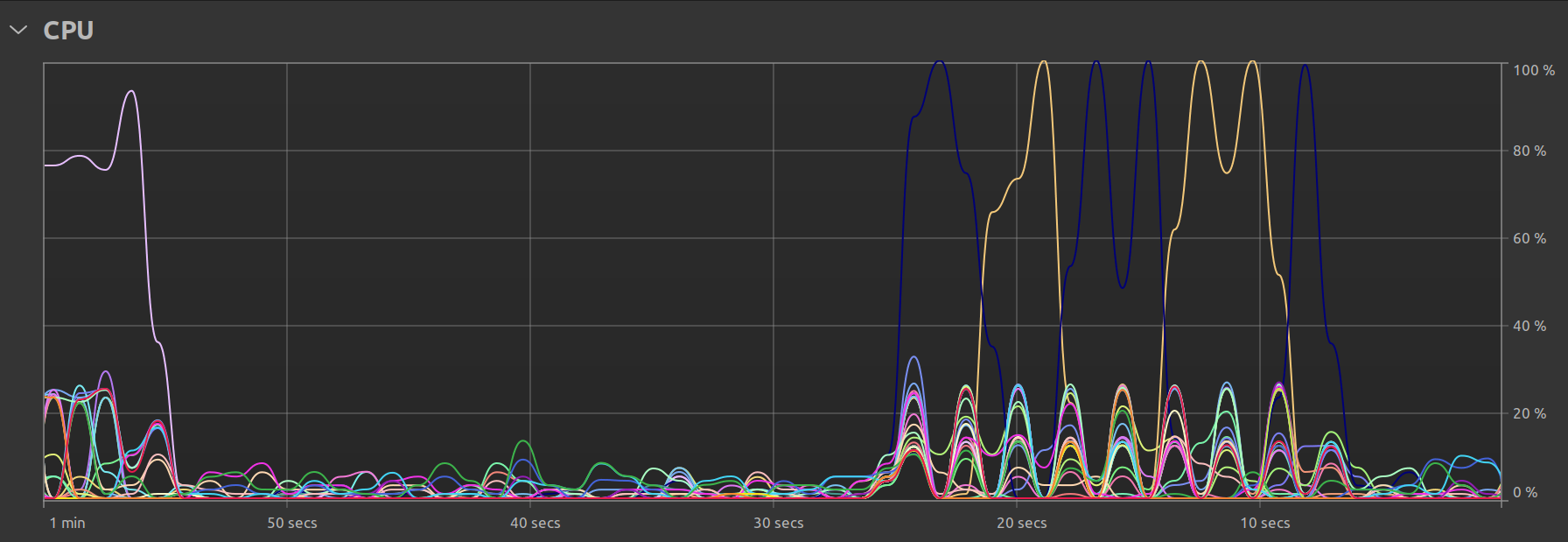
One final observation is my Ubuntu system’s own resource utilization graph. In the single threaded case, we clearly see that there is some parallel activity at program startup, but the bulk of the time is spent with just one thread doing all the work:

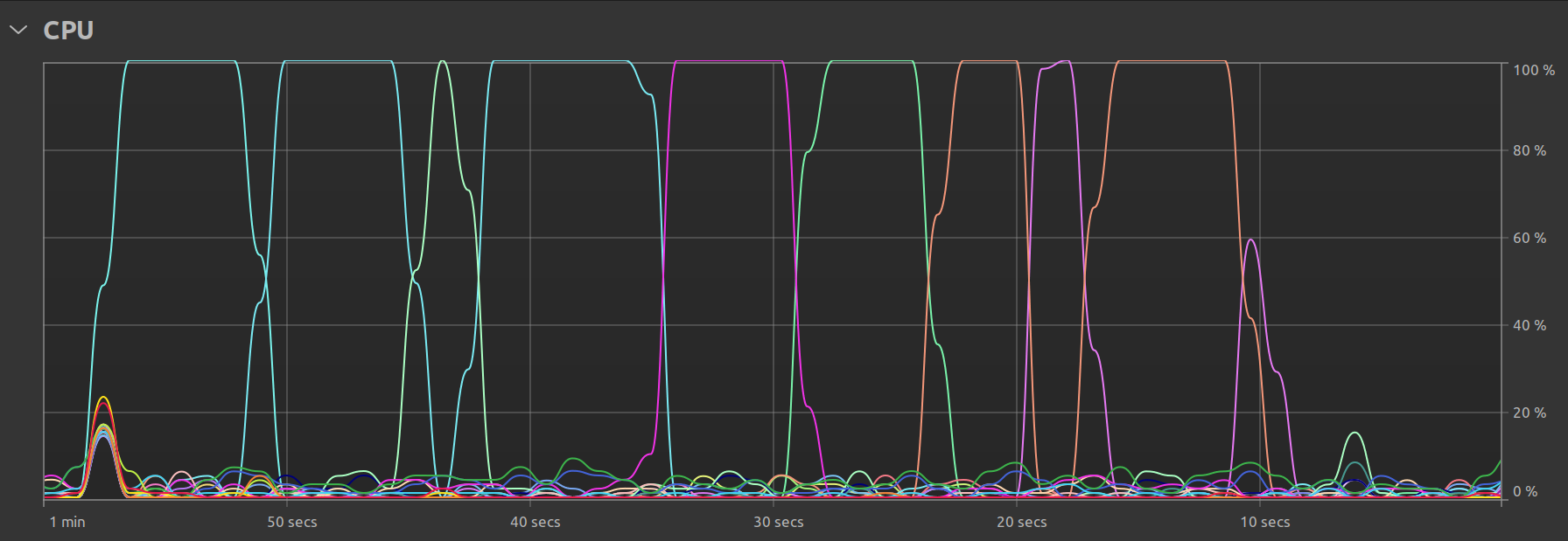
In the multi-threaded case, we can see that there is still one main thread but that there exist smaller “peaks” representing the times when the remaining available threads are called upon to perform the work:

Introduction:

My 2019 U.S. Patent, “Segmentation for Holographic Images” describes a method of 2D image segmentation that - when used as a precursor to 3D reconstruction algorithms - greatly improves resulting hologram photorealism relative to previously established prior art such as this landmark 2015 paper by Collet et al. The invention enhances augmented reality applications such as using human avatars for communication or preservation purposes. This technology was used by Microsoft’s Mixed Reality Capture Studios.

The following image shows the improvement in human avatar quality achieved with the described approach:

Summary:

I summarize the patent here by reviewing the ideas illustrated in the figures:

Figure 1 describes the relationship between volumetric 3D reconstruction and the 2D images: a 3D volume can be calculated from many 2D silhouettes. Thus, to accurately reconstruct a 3D volume observed in 2D images, many accurate volume silhouettes must be first obtained in 2D.

Because humans are extremely good at identifying other humans, producing human holograms with even slight volumetric errors is immersion-breaking for a consumer of augmented reality content. Figure 2 communicates that previous techniques used to obtain silhouettes were not sufficiently accurate for volumetric hologram applications at the time of this patent’s writing. In the absence of extremely well-labeled and diverse training data, even neural networks did not produce silhouettes accurate enough for human hologram applications. Traditional segmentation techniques like background subtraction are also defeated when the RGB intensities of background pixels are very similar to the RGB intensities of the target volume.

Figure 3 describes the approach proposed in this patent: combining (1) foreground-background subtraction, (2) neural network based semantic segmentation, and (3) statistical learning based postprocessing to produce highly refined silouettes for volumetric reconstruction.

Figure 5 outlines the algorithm pipeline proposed in this patent in text form:

Figure 6 shows the final payoff of the proposed approach in terms of hologram quality. The top image is an input to the hologram reconstruction algorithm described by Collet et al. The lower left image is a view of the hologram that is produced with traditional silhouette calculation approaches. The lower right image is a view of the hologram that is produced using the approach described in this patent. The improvement in reconstruction quality is drastic.

Description:

This PDF presentation is a talk I have given at several venues that provides an overview of the topic of dense 3D surface reconstruction 2D images. It includes 30 literature references on subtopics of the overview including many landmark papers in computer vision. The presentation covers both theory and implementation aspects of 3D surface reconstruction including discussions on camera calibration, disparity estimation, and 3D point cloud generation.

Teaser Image:

Description:

This .PDF technical report describes the mathematics theory and programming implementation of Gaussian Mixture Models and Expectation Maximization applied to image segmentation. I found myself needing to implement an image segmentation algorithm, but did not have the requisite training data to reproduce state-of-the-art methods in the domain. This motivated me to study the application of Gaussian Mixture Models, a classical machine learning approach that - while unable to produce state-of-the-art results - is fully unsupervised and does not require training data. The accompanying Python reference implementation is available on my GitHub page.

Teaser Image:

Description:

I created this GitHub repository where I write solutions to (most) problems in the popular computer science interview textbook, Cracking the Coding Interview, in Python and C++. The repository is differentiated by a high level of engineering rigor: the solutions have > 90% unit test coverage and an automatic build and testing system that compiles and verifies every solution. This project has gained the most public attention of any of my work on GitHub: it has over 500 stars, > 100 forks, and a place in the first page GitHub search results for the title of the textbook.

Description:

Autonomy is essential for flying on Mars because it’s impossible to remotely operate a flying vehicle due to the communications delay between planets. At a high level, the vehicle must calculate its change in pose over time at a high framerate (“odometry”). Over the summer I integrated a state-of-the-art visual odometry technique into NASA’s Mars exploration UAV prototype. This technique, Semi-Direct Visual Odometry by Forster et al, allows for the vehicle to be localized with centimeter accuracy using only information from a camera facing the surface of the planet. Solving the localization problem paves the way for autonomous navigation and exploration. In the video above, I briefly overview the technologies I integrated to achieve camera-only localization in a simulated Mars environment. In this video, I explain the project in detail during a technical talk at NASA. This PDF presentation contains the latest version of the slides.

Teaser Image: